The CFA Level II exam, administered by CFA Institute, is designed for investment professionals seeking to deepen their expertise in financial analysis and portfolio management. This exam validates your ability to apply investment tools and concepts to real-world scenarios, moving beyond foundational knowledge to practical decision-making. CFA Level II Chartered Financial Analyst candidates must demonstrate competency across ten core domains and synthesize knowledge across multiple areas. This page outlines the exam structure, syllabus, and effective preparation strategies to help you build confidence and readiness.
Use this topic map to guide your study for CFA Institute CFA-Level-II (CFA Level II Chartered Financial Analyst) within the CFA Level II path.
CFA Level II employs vignette-based items (scenario questions) that test both conceptual understanding and analytical reasoning in realistic contexts. The exam measures your ability to synthesize knowledge across topics and make sound investment decisions under ambiguity.
Effective preparation for CFA-Level-II requires structured study mapped to the ten core domains, combined with regular practice and review cycles. A typical candidate benefits from 300+ hours of focused study spread across 4-6 months, with emphasis on vignette practice and weak-area remediation.
Explore other CFA Institute certifications: view all CFA Institute exams.
Strengthen your preparation with up-to-date resources from validexamdumps.com. These materials align to CFA-Level-II and cover practical scenarios with clear explanations.
Visit the exam page to download the PDF, Online Practice Test, or get a bundle discount for both formats: CFA Level II Chartered Financial Analyst.
Portfolio Management and Wealth Planning, Equity Investments, and Fixed Income typically account for the largest portion of the exam. However, all ten domains are tested, and questions often integrate multiple topics. Allocate study time proportionally but ensure competency across all areas, as vignettes may test unexpected combinations.
In practice, investment professionals use all domains together: economic analysis informs asset allocation, financial statement analysis supports equity selection, derivatives hedge portfolio risk, and ethics guide every decision. CFA Level II vignettes simulate this integration by presenting scenarios where you must apply multiple frameworks. Understanding these connections deepens retention and improves your ability to answer complex questions.
Frequent errors include misreading vignette details (leading to incorrect analysis), applying the wrong valuation model without justifying the choice, and overlooking ethical dimensions of investment decisions. Candidates also struggle with time management and rush through calculations, introducing arithmetic errors. Slow down during practice to build accuracy; speed comes naturally with repetition.
In the final week, focus on review and confidence-building rather than learning new material. Re-solve vignettes from your weakest domains, review formula sheets and key definitions, and complete one final timed mock exam to assess readiness. Ensure adequate sleep, light exercise, and stress management in the days before the test to arrive mentally sharp.
CFA Level II assumes you have passed Level I and possess foundational knowledge; prior work experience in finance accelerates learning but is not required. Candidates without investment backgrounds often succeed by investing extra study time in practical application (working through case studies and vignettes) and seeking mentorship from experienced professionals. Focus on understanding frameworks and their real-world use rather than memorizing definitions.
Bill Henry, CFA, is the CIO of IS University Endowment Fund located in the United States. The Fund's total assets are valued at $3.5 billion. The investment policy uses a total return approach to meet the return objective that includes a spending rate of 5%. In addition, the policy constraints established make tax-exempt instruments an inappropriate investment vehicle. The Fund's current asset mix includes an 18% allocation to private equity. The private equity allocation is shown in Exhibit 1.
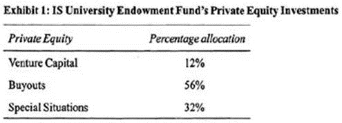
The private equity allocation is a mixture of funds with different vintages. For example, within the venture capital category, investments have been made in five different funds. Exhibit 2 provides detail about the Alpha Fund with a vintage year of 2006 and committed capital of SI95 million.
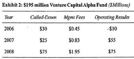
The Alpha Fund is considering a new investment in Targus Company. Targus is a start-up biotech company seeking $9 million of venture capital financing. Targus's founders believe that, based on the company's new drug pipeline, a company value of $300 million is reasonable in five years. Management at Alpha Fund views Targus Company as a risky investment and is using a discount rate of 40%. After a thorough analysis of Targus's future prospects, Alpha Fund's management believes that there is a possible 15% risk of failure for the company.
Which of the following is most likely a characteristic of a venture capital fund?
Venture capira! investments require considerable capital to develop and grow. Companies that require venture capital usually have significant cash burn as they develop new products. Venture capital investments arc ptimarily funded through equity and utilize little or no debt. Risk measurement of venture capital investments is difficult because of their short operating history, and the required development of new markets and technologies. (Study Session 13, LOS 47.c)
Josh Atwell recently inherited a large sum of money and wants to invest a portion of the inheritance into a real estate investment that provides a tax shelter. Atwell wants to take a limited management role in the real estate investment, and avoid the expense of hiring professional project management. Also, Atwell requires that the real estate investment generate high cash flows. Atwell hired Kellogg Investments to provide him potential real estate investments. Kellogg created Exhibit 1 outlining alternative real estate investments, from which Atwell can make his selection. Atwell's cost for any loan is 8%. The loan would be amortized over 20 years with annual payments. His required rate of return is 11%.
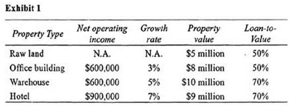
After reviewing the potential real estate investments generated by Kellogg, Atwell decided against all of the choices. Instead, Atwell requested a detailed report on the investment merits of an apartment complex. In Exhibit 2, Kellogg details the operating income of a targeted apartment complex investment. Atwell will make an equity contribution of $1,000,000. The loan-to-value ratio for the apartment complex investment would be 75%.
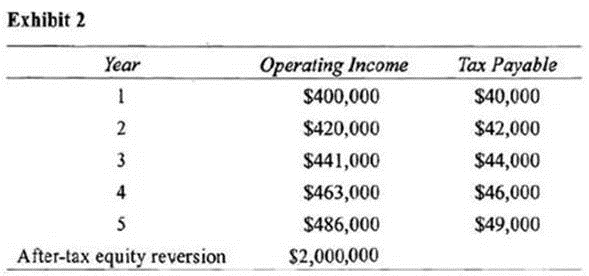
An adviser from Kellogg states that Atwell should purchase the apartment complex because the net present value of the investment is positive. The adviser also states, however, that the investment's IRR is less than Atwell's required rate of return. After reviewing the historical financial statements of the potential hotel investment, the advisor notes its erratic net operating income. In fact, the hotel generated several years of growing cash flow followed by two negative years and then a return back to a positive cash flow.
Based on the historical financial statements of the hotel, which of the following valuation techniques would be most appropriate?
If a real estate property's cash flow fluctuates, the best valuation approach is the net present value. IRR analysis of real estate investments has a number of limitations including multiple solutions when the investment has positive cash flow one year and a negative cash flow the next year. The direct capitalization approach is best used when the investments net operating income is stable. (Study Session 13, LOS 45-d and 46.d)
Factor Analytics Capital Management makes portfolio recommendations using various factor models. Mauricio Rodriguez, a Factor Analytics research analyst, is examining the prospects of two portfolios, the FACM Century Fund (CF) and the FACM Esquire Fund (EF).
The variance of returns are identical for the two funds. The estimates in Exhibit 1 were derived for CF and EF using monthly data for the past five years.
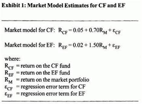
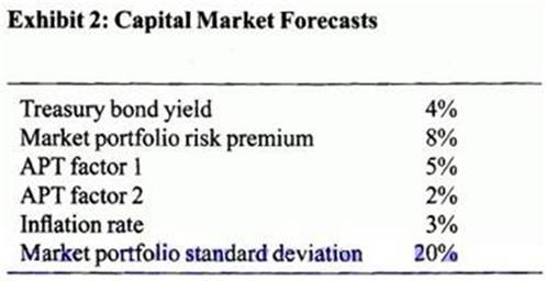
Supervisor Barbara Woodson asks Rodriguez to use the Capita! Asset Pricing Model (CAPM) and a multifactor model (APT) to make a decision to continue or discontinue the EF fund. The two factors in the multifactor model are not identified. To help with the decision, Woodson provides Rodriguez with the capital market forecasts in Exhibit 2.
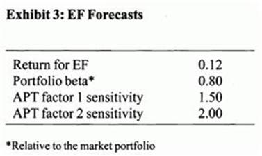
After examining the prospects for the EF portfolio, Rodriguez derives the forecasts in Exhibit 3.
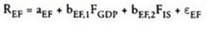
Rodriguez also develops a 2-factor macroeconomic factor model for the EF portfolio. The two factors used in the model are the surprise in GDP growth and the surprise in Investor Sentiment. The equation for the macro factor model is:

During an investment committee meeting, Woodson makes the following statements related to the 2-factor macroeconomic factor model.
Statement 1: An investment combination in CF and EF that provides a GDP growth factor beta equal to one and an Investor Sentiment factor beta equal to zero will have lower active factor risk than a tracking portfolio consisting of CF and EF.
Statement 2: When markets are in equilibrium, no combination of CF and EF will produce an arbitrage opportunity
In their final meeting, Rodriguez informs Woodson that the CF portfolio consistently outperformed its benchmark over the past five years. Rodriguez makes the following comments to Woodson: "The consistency with which CF outperformed its benchmark is amazing. The difference between the CF monthly return and its benchmark return was nearly always positive and varied little over time."
The intercept for the 2-factor macroeconomic model employed by Rodriguez for the EF portfolio, using the GDP growth and Investor Sentiment risk factors, is closest to:
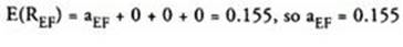
Macrocconomic factor models assume thai asset returns are explained by surprises (or 'shocks') in macroeconomic risk factors (e.g., GDP growth and Investor Sentiment). A factor surprise is defined as the difference between the realized value of the factor and its expected value, which is the expected return from the APT model (0.155 from Question 8). Therefore, the intercept must equal the expected return on the portfolio.
The equation for the macroeconomic factor model employed by Factor Analytics Capital Management is:
where the expected values of both factors are zero, and the expected value of the error term also is zero. Therefore, when markets move as expected:
(Study Session 18, LOS64.J)
Nigel Holmes, CFA, is an investment manager for a small money management firm in London. All of Holmes' clients are citizens of the U.K. Holmes urges all of his clients to maintain internationally diversified portfolios. In his efforts to find undervalued securities, he is currently analyzing a Canadian company called Slapshot, Inc. Slapshot produces hockey equipment at its Canadian manufacturing facilities. About 85% of Slapshot's sales are to the U .S . market, and the remainder are domestic (i.e., in Canada). Sales have been growing at 12% per year. Last year's sales were C$68,000,000. Holmes has gathered the following market information (inflation is perfectly predictable):
* /$ spot exchange rate = 0.8
* /C$ spot exchange rate = 0.4
* U.K. risk-free rate = 6%
* U.K. expected inflation rate = 4%
* Canadian risk-free rate = 9%
* Canadian expected inflation rate = 7%
* U .S . risk-free rate = 4%
* U .S . expected inflation = 2%
Holmes uses the international CAPM (ICAPM) to value international investments. For Slapshot, Holmes believes that the stock's returns are sensitive to the /C$ exchange rate. In order to apply the model, he estimates the following parameters using the as the base currency:
* World market risk premium = 6%
* Sensitivity of Slapshot to the world market = 1.2
* Sensitivity of Slapshot to changes in the /C$ exchange rate = 1.4
* Holmes' expectation for the depreciation of the C$ against the = 2%
* The ratio of the price of the U.K. consumption basket to the Canadian consumption basket is 0.3.
Holmes adds Slapshot stock to several client portfolios at a purchase price of C$ 100. One year later, the stock is trading at C$ 122. There were no dividend payments during the year.
Consider the current U .S . dollar to C$ ($/C$) spot exchange rate. Suppose that after one year, the nominal spot $/C$ exchange rate is 0.350. The most likely impact on Slapshot's valuation from the $/C$ exchange rate change is the:
Since the beginning-of-period $/C$ spot exchange rate is not given directly, we must calculate it from the /$ and /C$ quotes. Dividing /C$ by /$ gives a rate for the $/C$ exchange rate of 0.5. Next we need to determine whether there was any real change in the exchange rate during the year. Inflation in the United States is 2%, and inflation in Canada is 7% (remember that inflation is perfectly predictable). The 5% inflation differential means that to maintain parity, the C$ must depreciate by 5%. If the C$ depreciates by 5%, the new exchange rate would be 0.5(1 - 0.05) = 0.475. Since the end-of-period rate is less than what was expected given the inflation differential, the real value of the C$ has decreased. Hence, the firm should have a higher value because it is primarily an exporter, and exporters are helped by real domestic currency depreciation. (Study Session 18, LOS 66.e,m)
Wendall Wayne is a fixed income portfolio manager with Skyline Investments. Until recently he has focused almost exclusively on residential mortgage-backed securities (MBS). However, two weeks ago he was given approval to begin purchasing asset-backed securities (ABS) and commercial MBS as well. Wayne has forecasted that interest rates will decrease by approximately 100 basis points over the next month.
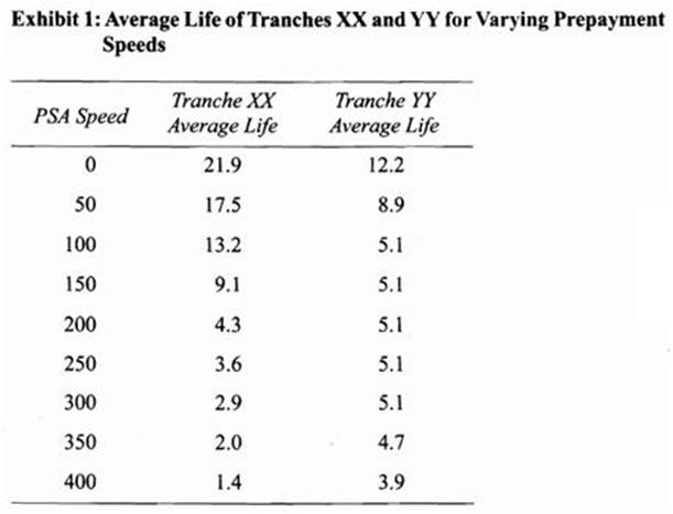
Wayne first completes an analysis of two tranches (a PAC I tranche and a support tranche) from a collateralized mortgage obligation (CMO) that was issued 18 months ago. When the CMO was issued, the initial collar of the PAC I tranche was 150 - 400 PSA . He estimates the change in the average life of each tranche as the prepayment speed varies, assuming the prepayment speed stays at that speed until the tranche matures. The results are shown in Exhibit 1.
In his report, Wayne makes the following statements regarding the CMO:
Statement 1: The CMO is structured so that the support tranche has more extension risk, and the PAC I tranche has more contraction risk.
Statement 2: The cash flows of the PAC I tranche will be less affected by the change in interest rates I have forecast than the cash flows of the support tranche.
Wayne has pushed for approval to begin trading ABS because he is particularly interested in collateralized debt obligations (CDOs). However, he doesn't know a lot about them, so he first does some reading and prepares some key points related to CDOs to guide his analysis.
Statement 3: CDOs are typically collateralized by emerging market bond issues, home equity bank loans, and high-yield corporate bond issues.
Statement 4: One advantage of issuing a synthetic CDO versus a cash CDO is that credit risk is lower with a synthetic CDO because the junior note holders also sell a credit default swap.
Statement 5: Some CDOs include an equity tranche to provide payment and credit protection to the senior and mezzanine tranches, but for most issues, credit protection is provided by external credit enhancements.
Wayne wants to understand the distinction between amortizing and non-amortizing assets that are securitized by ABS transactions, as well as the appropriate spread measures to use for various types of fixed-income securities. He asks a colleague, Martin Freed, to explain to him the difference between the two and how the payment structure of the ABS is affected by whether the assets in the pool are amortizing or non-amortizing. Freed replies:
Statement 6: An auto loan is an example of an amortizing asset, and a credit card receivable is an example of a non-amortizing asset.
Statement 7: For amortizing assets, the composition of the loans in the asset pool doesn't change once the assets are securitized. For non-amortizing assets, the composition of the asset pool does change.
Freed also tells Wayne that the credit analysis of commercial mortgage-backed securities (CMBS) should focus on the credit risk of the property, not the borrower. Freed also says that two key ratios useful for assessing the credit risk of the property are the debt service coverage ratio (net operating income/debt service) and the loan-to-value ratio (current mortgage amount/current appraised value). Wayne concludes that both of the ratios Freed recommends for credit analysis of CMBS are positively related to credit risk: the higher the ratio, the more risky the loan.
Finally, Wayne is trying to determine the most appropriate spread measure for valuing callable corporate bonds and high-quality home equity loan ABS. He plans to choose from the following measures: the zero-volatility spread, the OAS from the binomial model, and the OAS from the Monte Carlo model.
Is Wayne correct or incorrect with regard to his analysis of debt service coverage and loan-to-value?
Wayne is incorrect with respect to the debt service coverage ratio because the higher the ratio, the lower the credit risk. Wayne is correct with respect to the loan-io-value ratio because the higher the ratio, the higher the credit risk. {Study Session 15, LOS 55.1)